Finding Viable Parameter Spaces with Sensitivity Analysis
yuval bloch
Introduction
Ecological models often depend on parameters that are difficult to measure precisely. Sensitivity analysis helps us ask: how much do these uncertainties matter? It allows us to explore:
-
Which parameters most strongly influence model outcomes
-
What combinations lead to persistence or extinction
-
How robust the system is to changes in key assumptions
In this project, I go beyond simply measuring sensitivity. I use these tools to map the boundary between viable and non-viable ecological conditions—the tipping points where tick populations either collapse or persist. By comparing these boundaries to patterns observed in real-world data, I can ask a deeper question: which combinations of parameters are not just viable, but actually relevant to the system I’m trying to model?
Types of Sensitivity Analysis
Throughout this work, I use several types of sensitivity analysis, each suited to a specific goal:
❌ Local Sensitivity Analysis
Changes one parameter at a time.
Not used here—interactions between parameters are too strong for this to be meaningful.
🌍 Regional Sensitivity Analysis
Explores combinations of a few key parameters.
Used to locate regions where ticks either survive or go extinct under plausible ecological assumptions.
🌐 Global Sensitivity Analysis
Covers the full parameter space.
Used to identify dominant parameters and how they interact across the entire model.
🏞 Structural Sensitivity Analysis
Varies landscape structure instead of parameters.
Used to test how spatial patterns (e.g. land use maps) affect tick dynamics.
Covered separately due to complexity.
Using SVM to Define the Viable Parameter Space
The first task was to identify which combinations of ecological parameters allow tick populations to persist. I focused on three key ones:
k: Carrying capacityd₀: Death rate when ticks are rared_c: Death rate at carrying capacity
I ran many simulations with randomly sampled values for these parameters, labeling the outcomes:
0: Population went extinct1: Population persisted
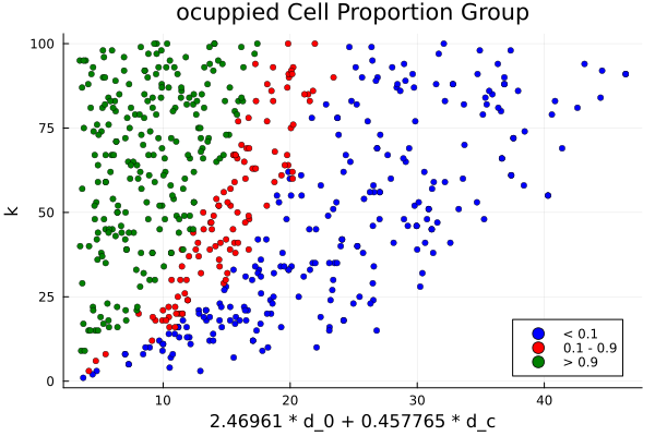
To organize and generalize these results, I trained a Support Vector Machine (SVM). Rather than just speeding things up, the SVM became central: it learned the boundary between survival and extinction and gave me a functional representation of the viable region in parameter space.
Active Learning: Smarter Sampling
To improve the SVM with fewer simulations, I used active learning. The model identified parameter sets near the decision boundary—where it was most uncertain—and I focused simulations there.
I tried a few kernel functions and settled on a polynomial kernel, which captured the nonlinear shape of the viability boundary best.
Beyond Viability: Exploring System Behavior
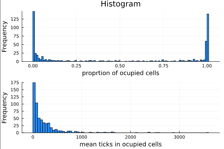
Once I mapped the viability zone, I looked more closely at how the model behaves across it. I used three summary statistics:
- Proportion of occupied cells
- Mean number of ticks per occupied cell
- Overall average tick density
Many parameter sets produced all-or-nothing results—either nearly all cells were full or nearly all were empty. But real ecosystems aren’t so binary. I was looking for mixed outcomes: some patches full, others not. This is what I observed in field data and wanted the model to reflect.
Parameter Insights
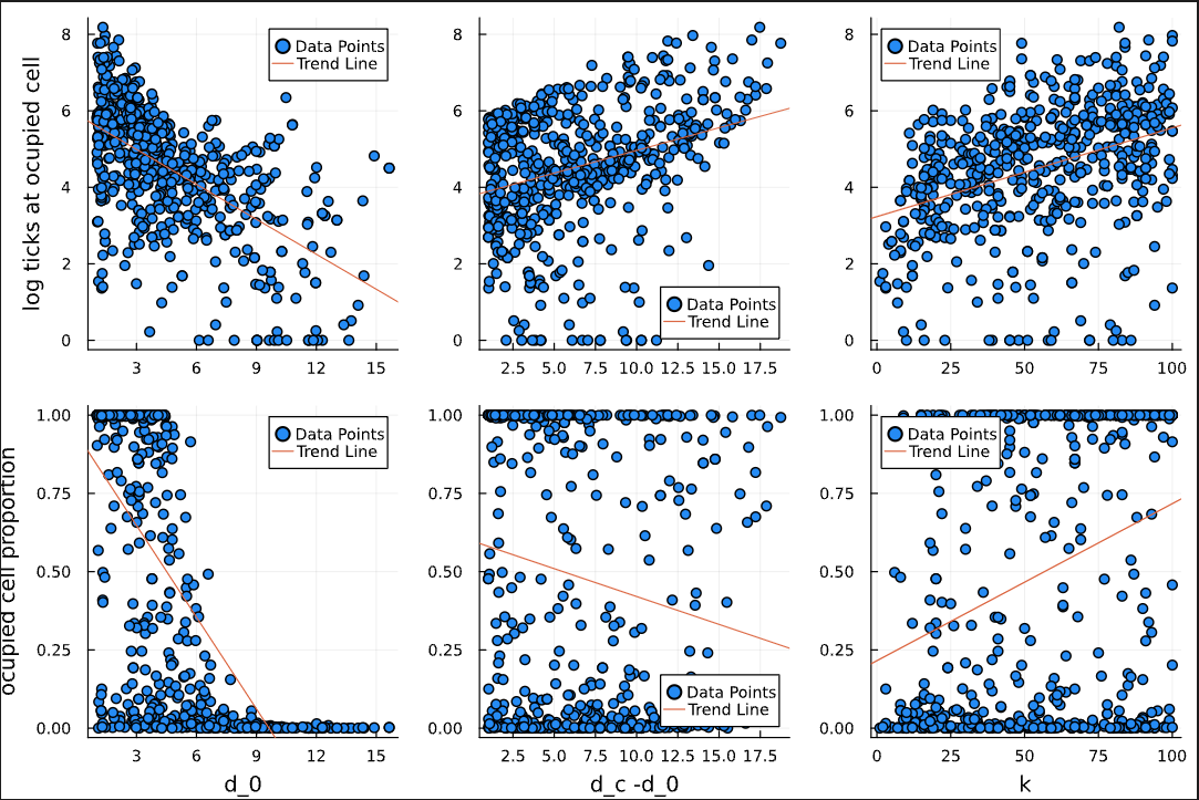
Looking across the viable space, several patterns became clear:
-
Increasing
d₀reduces both:- The proportion of occupied cells
- The average number of ticks per occupied cell
-
Increasing
khas the opposite effect:- It raises both patch occupancy and tick density
-
The difference between
d₀andd_calso matters:- A larger difference boosts the number of surviving patches
- But lowers the average tick count within them—possibly due to early saturation
What I’m Looking For
The real world is not homogeneous. Field data show variation—some areas have ticks, others do not—and this pattern holds across different values of k. To reflect that, I searched for parameter sets that produced:
-
Heterogeneous landscapes with partial tick occupancy
-
Moderate tick densities that avoid unrealistic overpopulation
After testing many combinations, I identified one that struck a good balance. Tick populations persisted in some areas while remaining ecologically realistic, closely aligning with observed dynamics.
The final question I need to answer before applying this model to real land use scenarios is whether it responds only to average carrying capacity—or if it’s also sensitive to the structure of the landscape itself. This matters because research shows that spatial structure can strongly influence tick populations, yet it’s much harder to capture in models.
In my next post, I’ll explore this by using a beautiful mathematical concept: fractal dimensionality. I’ll show how it reveals that the model isn’t just reacting to average conditions—it’s truly sensitive to the spatial complexity of the land.
📢 Stay tuned—it gets surprisingly elegant.